GPT_CONFIG_124M = {
    "vocab_size": 50257,    # vocabulary size
    "context_length": 1024, # context length
    "emb_dim": 768,         # embedding dimension
    "n_heads": 12,          # number of attention heads
    "n_layers": 12,         # number of layers
    "drop_rate": 0.1,       # dropout rate
    "qkv_bias": True,       # whether to use bias in the query, key, and value projections
}GPT model from scratch
llm
Configuration
First we need to specify the configurations of the small GPT-2 model.
where each key is:
vocab_size: the size of the vocabulary, as used by the BPE tokenizercontext_length: the maximum number of tokens that the model can handle via positional embeddingsemb_dim: the embedding size, transforming each token into a 768-dimensional vectorn_heads: the count of attention heads in the multi-head attention mechanismn_layers: number of transformer blocks in the modeldrop_rate: the dropout rate for the attention mechanismqkv_bias: whether to use bias in the query, key, and value projections
A placeholder GPT model architecture class
import torch
import torch.nn as nn

class DummyGPTModel(nn.Module):
    def __init__(self, config):
        super().__init__()
        self.tok_emb = nn.Embedding(config["vocab_size"], config["emb_dim"])
        self.pos_emb = nn.Embedding(config["context_length"], config["emb_dim"])
        self.drop_emb = nn.Dropout(config["drop_rate"])
        self.trf_blocks = nn.Sequential(
            *[DummyTransformerBlock(config) for _ in range(config["n_layers"])]
        )
        self.final_norm = DummyLayerNorm(config["emb_dim"])
        self.out_head = nn.Linear(config["emb_dim"], config["vocab_size"], bias=False)

    def forward(self, in_idx):
        batch_size, seq_len = in_idx.shape
        tok_embeds = self.tok_emb(in_idx)
        pos_embeds = self.pos_emb(
            torch.arange(seq_len, device=in_idx.device)
        )

        x = tok_embeds + pos_embeds
        x = self.drop_emb(x)
        x = self.trf_blocks(x)
        x = self.final_norm(x)
        logits = self.out_head(x)
        return logits
Transformer architecture
class DummyTransformerBlock(nn.Module):
    def __init__(self, config):
        super().__init__()

    def forward(self, x):
        return x

class DummyLayerNorm(nn.Module):
    def __init__(self, normalized_shape, eps=1e-5):
        super().__init__()

    def forward(self, x):
        return x
Preparing data
import tiktoken

tokenizer = tiktoken.get_encoding("gpt2")
batch = []

txt1 = 'Every effort moves you'
txt2 = 'Every day holds a'

batch.append(torch.tensor(tokenizer.encode(txt1)))
batch.append(torch.tensor(tokenizer.encode(txt2)))
batch = torch.stack(batch, dim=0)
print(batch)
tensor([[6109, 3626, 6100, 345],
[6109, 1110, 6622, 257]])Now that we have a (tokenized) input data, we can feed it into our 124M GPT-2 model:
torch.manual_seed(123)
model = DummyGPTModel(GPT_CONFIG_124M)
logits = model(batch)
print("Output shape:", logits.shape)
print("Output:", logits)
Output shape: torch.Size([2, 4, 50257])
Output: tensor([[[-1.2034, 0.3201, -0.7130, ..., -1.5548, -0.2390, -0.4667],
[-0.1192, 0.4539, -0.4432, ..., 0.2392, 1.3469, 1.2430],
[ 0.5307, 1.6720, -0.4695, ..., 1.1966, 0.0111, 0.5835],
[ 0.0139, 1.6754, -0.3388, ..., 1.1586, -0.0435, -1.0400]],
[[-1.0908, 0.1798, -0.9484, ..., -1.6047, 0.2439, -0.4530],
[-0.7860, 0.5581, -0.0610, ..., 0.4835, -0.0077, 1.6621],
[ 0.3567, 1.2698, -0.6398, ..., -0.0162, -0.1296, 0.3717],
[-0.2407, -0.7349, -0.5102, ..., 2.0057, -0.3694, 0.1814]]],
grad_fn=<UnsafeViewBackward0>)Normalizing activations with layer normalization
We now implement layer normalization to improve training stability and efficiency of neural network training. The main idea behind normalization is to adjust the activation outputs to have mean 0 and variance 1 (also known as unit variance).
torch.manual_seed(123)
batch_example = torch.randn(2, 5)
layer = nn.Sequential(nn.Linear(5,6), nn.ReLU())
out = layer(batch_example)
print(out)

# examine the mean and variance of the output
print("Mean:", out.mean(dim=-1, keepdim=True))
print("Variance:", out.var(dim=-1, keepdim=True))
tensor([[0.2260, 0.3470, 0.0000, 0.2216, 0.0000, 0.0000],
[0.2133, 0.2394, 0.0000, 0.5198, 0.3297, 0.0000]],
grad_fn=<ReluBackward0>)
Mean: tensor([[0.1324],
[0.2170]], grad_fn=<MeanBackward1>)
Variance: tensor([[0.0231],
[0.0398]], grad_fn=<VarBackward0>)Let’s now apply layer normalization to the layer outputs we obtained earlier. The operation consists of subtracting the mean and dividing by the standard deviation of the activation outputs.
mean = out.mean(dim=-1, keepdim=True)
var = out.var(dim=-1, keepdim=True)

out_norm = (out - mean) / torch.sqrt(var)
mean = out_norm.mean(dim=-1, keepdim=True)
var = out_norm.var(dim=-1, keepdim=True)
print("Normalized output:", out_norm)
print("Mean:", mean)
print("Variance:", var)
Normalized output: tensor([[ 0.6159, 1.4126, -0.8719, 0.5872, -0.8719, -0.8719],
[-0.0189, 0.1121, -1.0876, 1.5173, 0.5647, -1.0876]],
grad_fn=<DivBackward0>)
Mean: tensor([[-5.9605e-08],
[ 1.9868e-08]], grad_fn=<MeanBackward1>)
Variance: tensor([[1.0000],
[1.0000]], grad_fn=<VarBackward0>)With that, we can implement a proper layer normalization class:
class LayerNorm(nn.Module):
    def __init__(self, emb_dim):
        super().__init__()
        self.eps = 1e-5  # small constant to avoid division by zero
        self.scale = nn.Parameter(torch.ones(emb_dim))   # learnable per-feature stretch (γ)
        self.shift = nn.Parameter(torch.zeros(emb_dim))  # learnable per-feature shift (β)

    def forward(self, x):
        mean = x.mean(dim=-1, keepdim=True)
        var = x.var(dim=-1, keepdim=True, unbiased=False)
        norm_x = (x - mean) / torch.sqrt(var + self.eps)
        return self.scale * norm_x + self.shift  # restore representational flexibility after normalization
Let’s now apply layer normalization to the layer outputs we obtained earlier.
ln = LayerNorm(emb_dim=5)
out_ln = ln(batch_example)
mean = out_ln.mean(dim=-1, keepdim=True)
var = out_ln.var(dim=-1, keepdim=True, unbiased=False)
print("Normalized output:", out_ln)
print("Mean:", mean)
print("Variance:", var)
Normalized output: tensor([[ 0.5528, 1.0693, -0.0223, 0.2656, -1.8654],
[ 0.9087, -1.3767, -0.9564, 1.1304, 0.2940]], grad_fn=<AddBackward0>)
Mean: tensor([[-2.9802e-08],
[ 0.0000e+00]], grad_fn=<MeanBackward1>)
Variance: tensor([[1.0000],
[1.0000]], grad_fn=<VarBackward0>)Implementing a FFN with GELU activations
GELU activation function
The GELU function is defined as \(\text{GELU}(x) = x \Phi(x)\) where \(\Phi(x)\) is the cumulative distribution function of the standard normal distribution. However, in practice, it’s common to approximate the GELU function with a simpler expression (GPT-2 was also trained with this approximation version), which could be expressed as follows:
\[ \text{GELU}(x) = x \Phi(x) \approx 0.5x(1 + \tanh(\sqrt{2/\pi}(x + 0.044715x^3))) \]
In code, we could implement it as:
class GELU(nn.Module):
    def __init__(self):
        super().__init__()

    def forward(self, x):
        return 0.5 * x * (1 + torch.tanh(torch.sqrt(torch.tensor(2.0 / torch.pi)) * (x + 0.044715 * x**3)))
We can plot ReLU and GELU activations to see the difference:
import matplotlib.pyplot as plt
gelu, relu = GELU(), nn.ReLU()

x = torch.linspace(-5, 5, 100)
y_gelu, y_relu = gelu(x), relu(x)
plt.figure(figsize=(10, 5))

for i, (y, label) in enumerate(zip([y_gelu, y_relu], ['GELU', 'ReLU']), 1):
    plt.subplot(1, 2, i)
    plt.plot(x, y)
    plt.title(f"{label} activation function")
    plt.xlabel("x")
    plt.ylabel("y")
plt.tight_layout()
plt.show()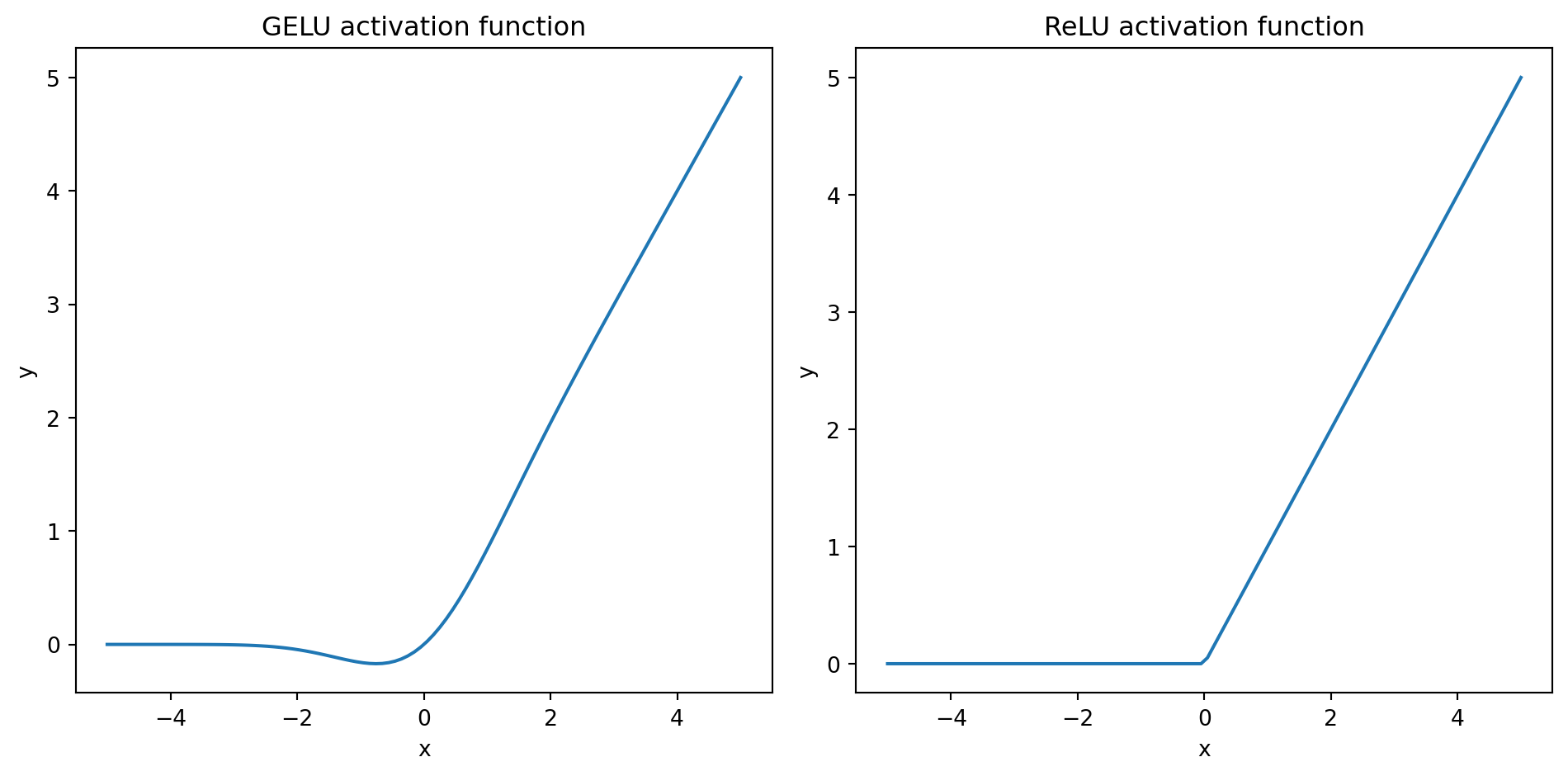
Feed-forward network
The feed forward neural network that we will implement is one that consists of two Linear layers and a GELU activation function.
class FeedForward(nn.Module):
    def __init__(self, cfg):
        super().__init__()
        self.layers = nn.Sequential(
            nn.Linear(cfg["emb_dim"], 4 * cfg["emb_dim"]),
            GELU(),
            nn.Linear(4 * cfg["emb_dim"], cfg["emb_dim"]),
        )

    def forward(self, x):
        return self.layers(x)
We can now use this as follows:
ffn = FeedForward(GPT_CONFIG_124M)
x = torch.rand(2,3,768)
out = ffn(x)
print(out.shape)
torch.Size([2, 3, 768])Adding shortcut connections
class ExampleDeepNeuralNetwork(nn.Module):
    def __init__(self, layer_sizes, use_shortcut):
        super().__init__()
        self.use_shortcut = use_shortcut
        self.layers = nn.ModuleList([
            nn.Sequential(nn.Linear(layer_sizes[0], layer_sizes[1]), GELU()),
            nn.Sequential(nn.Linear(layer_sizes[1], layer_sizes[2]), GELU()),
            nn.Sequential(nn.Linear(layer_sizes[2], layer_sizes[3]), GELU()),
            nn.Sequential(nn.Linear(layer_sizes[3], layer_sizes[4]), GELU()),
            nn.Sequential(nn.Linear(layer_sizes[4], layer_sizes[5]), GELU()),
        ])

    def forward(self, x):
        for layer in self.layers:
            layer_output = layer(x)
            if self.use_shortcut and x.shape == layer_output.shape:
                x = x + layer_output
            else:
                x = layer_output
        return x
Let’s now print out the gradients to check the training dynamics:
def print_gradients(model, x):

    output = model(x)                   # forward pass
    target = torch.tensor([[0.]])

    loss = nn.MSELoss()

    # calculate loss
    loss = loss(output, target)
    loss.backward()

    for name, param in model.named_parameters():
        if 'weight' in name:
            print(f"{name} has gradient mean of {param.grad.abs().mean().item()}")

layer_sizes = [3, 3, 3, 3, 3, 1]
sample_input = torch.tensor([[1., 0., -1.]])
torch.manual_seed(123)
model_without_shortcut = ExampleDeepNeuralNetwork(layer_sizes, use_shortcut=False)
model_with_shortcut = ExampleDeepNeuralNetwork(layer_sizes, use_shortcut=True)

print_gradients(model_without_shortcut, sample_input)
print("-"*50)
print_gradients(model_with_shortcut, sample_input)
layers.0.0.weight has gradient mean of 0.00020173587836325169
layers.1.0.weight has gradient mean of 0.0001201116101583466
layers.2.0.weight has gradient mean of 0.0007152041071094573
layers.3.0.weight has gradient mean of 0.0013988735154271126
layers.4.0.weight has gradient mean of 0.005049645435065031
--------------------------------------------------
layers.0.0.weight has gradient mean of 0.0014432291500270367
layers.1.0.weight has gradient mean of 0.004846951924264431
layers.2.0.weight has gradient mean of 0.004138893447816372
layers.3.0.weight has gradient mean of 0.005915115587413311
layers.4.0.weight has gradient mean of 0.032659437507390976Connecting attention and linear layers in a transformer block
![]()
We can implement a Transformer block as follows, where the Multi-head attention class is implemented in ?@lst-mha.
class TransformerBlock(nn.Module):
    def __init__(self, cfg):
        super().__init__()

        # we implement the multi-head attention class in previous section.
        self.attn = MultiHeadAttention(
            d_in=cfg["emb_dim"],
            d_out=cfg["emb_dim"],
            context_length=cfg["context_length"],
            dropout=cfg["drop_rate"],
            num_heads=cfg["n_heads"],
            qkv_bias=cfg["qkv_bias"]
        )
        self.ffn = FeedForward(cfg)
        self.norm1 = LayerNorm(cfg["emb_dim"])
        self.norm2 = LayerNorm(cfg["emb_dim"])
        self.drop_shortcut = nn.Dropout(cfg["drop_rate"])

    def forward(self, x):

        shortcut = x
        x = self.norm1(x)
        x = self.attn(x)
        x = self.drop_shortcut(x)
        x = x + shortcut

        shortcut = x
        x = self.norm2(x)
        x = self.ffn(x)
        x = self.drop_shortcut(x)
        x = x + shortcut
        return x
The transformer block maintains the input dimensions in its output, indicating that the transformer architecture processes sequences of data without altering their shape throughout the network.
torch.manual_seed(123)
x = torch.rand(2,4,768)
block = TransformerBlock(GPT_CONFIG_124M)
output = block(x)

print("Input shape: ", x.shape)
print("Output shape: ", output.shape)
Input shape: torch.Size([2, 4, 768])
Output shape: torch.Size([2, 4, 768])GPT Model architecture implementation
class GPTModel(nn.Module):
    def __init__(self, cfg):
        super().__init__()
        self.tok_emb = nn.Embedding(cfg["vocab_size"], cfg["emb_dim"])
        self.pos_emb = nn.Embedding(cfg["context_length"], cfg["emb_dim"])
        self.drop_emb = nn.Dropout(cfg["drop_rate"])

        self.trf_blocks = nn.Sequential(
            *[TransformerBlock(cfg) for _ in range(cfg["n_layers"])])
        self.final_norm = LayerNorm(cfg["emb_dim"])
        self.out_head = nn.Linear(cfg['emb_dim'], cfg['vocab_size'], bias=False)

    def forward(self, in_idx):
        batch_size, seq_len = in_idx.shape
        tok_embeds = self.tok_emb(in_idx)
        pos_embeds = self.pos_emb(
            torch.arange(seq_len, device=in_idx.device)
        )
        x = tok_embeds + pos_embeds
        x = self.drop_emb(x)
        x = self.trf_blocks(x)
        x = self.final_norm(x)
        logits = self.out_head(x)
return logits torch.manual_seed(123)
model = GPTModel(GPT_CONFIG_124M)
out = model(batch)
print("Input batch:", batch)
print("Output shape:", out.shape)
print("Output:", out)Input batch: tensor([[6109, 3626, 6100, 345],
[6109, 1110, 6622, 257]])
Output shape: torch.Size([2, 4, 50257])
Output: tensor([[[-0.4546, 0.0081, -0.3693, ..., -0.1397, -0.3408, -0.0404],
[ 0.5395, -0.5098, 1.0554, ..., -0.5960, -0.3028, -0.2684],
[ 0.0478, -0.2459, -0.3739, ..., -0.4117, -0.3174, -0.1074],
[ 0.0547, 0.3506, 0.4306, ..., -0.0702, 0.3131, 0.1302]],
[[-0.4348, -0.5515, -0.0093, ..., 0.0666, -0.3099, 0.0341],
[-0.2447, -0.8705, 1.5947, ..., -0.7661, -0.6889, 0.1404],
[-0.2036, -0.6698, -0.4476, ..., -0.1229, -0.8122, 0.4316],
[-0.0733, 1.2139, 0.2007, ..., -0.0809, -0.4936, -0.5157]]],
grad_fn=<UnsafeViewBackward0>)Let’s see the total number of parameters in the model:
total_params = sum(p.numel() for p in model.parameters())
print("Total number of parameters:", total_params)

# calculate the size
total_size_bytes = total_params * 4
total_size_mb = total_size_bytes / (1024 * 1024)
print("Total size in MB:", total_size_mb)
Total number of parameters: 163037184
Total size in MB: 621.9375Generating text
def generate_text_simple(model, idx, max_new_tokens, context_size):
    for _ in range(max_new_tokens):
        idx_cond = idx[:, -context_size:]
        with torch.no_grad():
            logits = model(idx_cond)

        logits = logits[:, -1, :]
        probas = torch.softmax(logits, dim=-1)
        idx_next = torch.argmax(probas, dim=-1, keepdim=True)
        idx = torch.cat((idx, idx_next), dim=1)

    return idx
Let’s try it out
start_context = 'Hello, I am'
encoded = tokenizer.encode(start_context)
print("encoded:", encoded)
encoded_tensor = torch.tensor(encoded).unsqueeze(0)
print("encoded_tensor:", encoded_tensor.shape)
encoded: [15496, 11, 314, 716]
encoded_tensor: torch.Size([1, 4])The next step is to put the model to eval() mode to disable random components like dropout (which are only used during training).
model.eval()

out = generate_text_simple(
    model = model,
    idx = encoded_tensor,
    max_new_tokens = 6,
    context_size = GPT_CONFIG_124M["context_length"]
    )

print("Output:", out)
print("Output length:", len(out[0]))
Output: tensor([[15496, 11, 314, 716, 3127, 29991, 6539, 21826, 18530, 6276]])
Output length: 10We can use the decode method to convert the encoded tokens back to text:
decoded = tokenizer.decode(out.squeeze(0).tolist())
print("Decoded:", decoded)
Decoded: Hello, I am network BEL Afghan postp aired technical